1. Executive Summary
This datasheet provides a technical evaluation of the Simthetic Hybrid Reduced Order Model (ROM) for a DCDC Buck Converter. The ROM was benchmarked against a high-fidelity MATLAB/Simscape reference across two stress-test scenarios (step load transient and combined line ramp + sinusoidal duty cycle modulation).
- Computational Speedup: Simthetic executes $28\times$ to $31\times$ faster than the Simscape solver.
- Output-side accuracy: Mean Absolute Error (MAE) on the output voltage ($V_{out}$) stays below $1.2\%$ of signal range; MAE on the output current ($I_{out}$) stays below $2.6\%$ across both scenarios.
- Deployment: The model ships as a self-contained Docker container with no MATLAB, PyTorch or GPU runtime dependencies, and the underlying ROM core compiles to a standalone C library (
.dll/.so) for embedded targets.
2. Test Methodology
Reference Solver (Simscape)
- Local solver: Backward Euler, fixed step $5 \times 10^{-7}\,\text{s}$
- Top-level Simulink solver: Variable-step (auto), default tolerances
- Sample time of logged signals: $\sim 5\,\mu s$ (interpolated to ROM grid for comparison)
Simthetic ROM
- Container:
simthetic/my-rom:v1 - Invocation: Single REST call per scenario via the on-host MCP / REST bridge
- Reported execution time: ROM-internal
elapsed_sfromsim.json(does not include container startup or HTTP round-trip)
Error Metrics
For each signal, the Simscape trace is linearly interpolated onto the ROM time grid and compared sample-by-sample. All percentages are normalised by the signal's peak-to-peak range over the scenario ($\max - \min$ of the reference). For approximately-constant signals (e.g. $V_{in}$ on Vector 1), the nominal magnitude is used as the normaliser instead.
| Symbol | Definition |
|---|---|
| MAE % | $\dfrac{1}{N} \sum \lvert e_k \rvert \,/\, \text{range} \cdot 100$ - average absolute error |
| RMSE % | $\sqrt{\tfrac{1}{N} \sum e_k^2} \,/\, \text{range} \cdot 100$ - root-mean-square error |
| MaxErr % | $\max_k \lvert e_k \rvert \,/\, \text{range} \cdot 100$ - single worst-sample deviation |
3. ROM Operating Range
The ROM was trained over the following parameter envelope. Behaviour outside this envelope is undefined; for new operating regions Simthetic recommends a re-fit.
| Channel | Min | Max | Units |
|---|---|---|---|
$V_{in,set}$ (Vin_int) | 10 | 45 | V |
$R_{load}$ (Rload_int) | 1 | 10 | $\Omega$ |
Duty cycle (DC_int) | 0.2 | 0.8 | — |
Both benchmark scenarios below sit fully inside this range, including the lower-boundary case ($R_{load} = 1\,\Omega$ in Vector 1).
4. Quantitative Accuracy
Vector 1 - Step Load Transient
Constant $V_{in} = 24\,\text{V}$, $DC = 0.5$. Load steps: $10\,\Omega \rightarrow 1\,\Omega$ at $t = 25\,\text{ms}$, $1\,\Omega \rightarrow 10\,\Omega$ at $t = 100\,\text{ms}$. Total duration $250\,\text{ms}$.
| Signal | MAE % | RMSE % | MaxErr % | Reference Range |
|---|---|---|---|---|
| $V_{out}$ | 0.52% | 2.24% | 58.20% ¹ | $36.25\,\text{V}$ |
| $I_{out}$ | 1.07% | 2.01% | 37.10% ¹ | $11.88\,\text{A}$ |
| $V_{in}$ | 0.86% | 0.99% | 10.20% | $24.0\,\text{V}$ (nominal) |
| $I_{in}$ | 4.75% | 11.52% | 285.08% ² | $6.19\,\text{A}$ |
Vector 2 - Line Ramp + Sinusoidal Duty Cycle
$V_{in}$ ramp $20\,\text{V} \rightarrow 40\,\text{V}$ over the first $100\,\text{ms}$, then held. $DC = 0.45 + 0.05 \sin(2\pi \cdot 100\,\text{Hz} \cdot t)$. $R_{load} = 5\,\Omega$ constant. Total duration $250\,\text{ms}$.
| Signal | MAE % | RMSE % | MaxErr % | Reference Range |
|---|---|---|---|---|
| $V_{out}$ | 1.17% | 1.68% | 26.84% ¹ | $19.95\,\text{V}$ |
| $I_{out}$ | 2.51% | 3.02% | 25.50% ¹ | $3.99\,\text{A}$ |
| $V_{in}$ | 0.28% | 0.45% | 1.79% | $20.00\,\text{V}$ |
| $I_{in}$ | 8.20% | 23.65% | 680.05% ² | $2.07\,\text{A}$ |
Notes on MaxErr % Spikes
¹ Switching-instant phase offset - At a step transition or sharp control event, the ROM produces its next sample one ROM-period ($50\,\mu s$) after the Simscape solver has already executed several sub-microsecond integration steps. The resulting two-trace misalignment produces a single-sample percent error that is large at the instant of the event but decays to <2% within a few hundred microseconds. As shown in the §5 waveform plots, the post-transient settling is in agreement with the reference.
² Input current ($I_{in}$) - small-range normalisation - $I_{in}$ has the smallest peak-to-peak range of all four signals ($6.19\,\text{A}$ for V1 and $2.07\,\text{A}$ for V2). Because the percentage error divides by that range, the same absolute error magnitude that produces 2–3% on $V_{out}$ produces a much larger number here. The absolute MAE on $I_{in}$ is $0.29\,\text{A}$ (V1) and $0.17\,\text{A}$ (V2). Customers using $I_{in}$ for power-balance or efficiency calculations should evaluate this against their target tolerance.
5. Visual Waveform Validation
The plots below compare the transient trajectories of the MATLAB/Simscape reference (solid black) and the Simthetic ROM (dashed red). The right column shows the per-sample error as a percentage of the reference signal range.
Vector 1 - Step Load Response
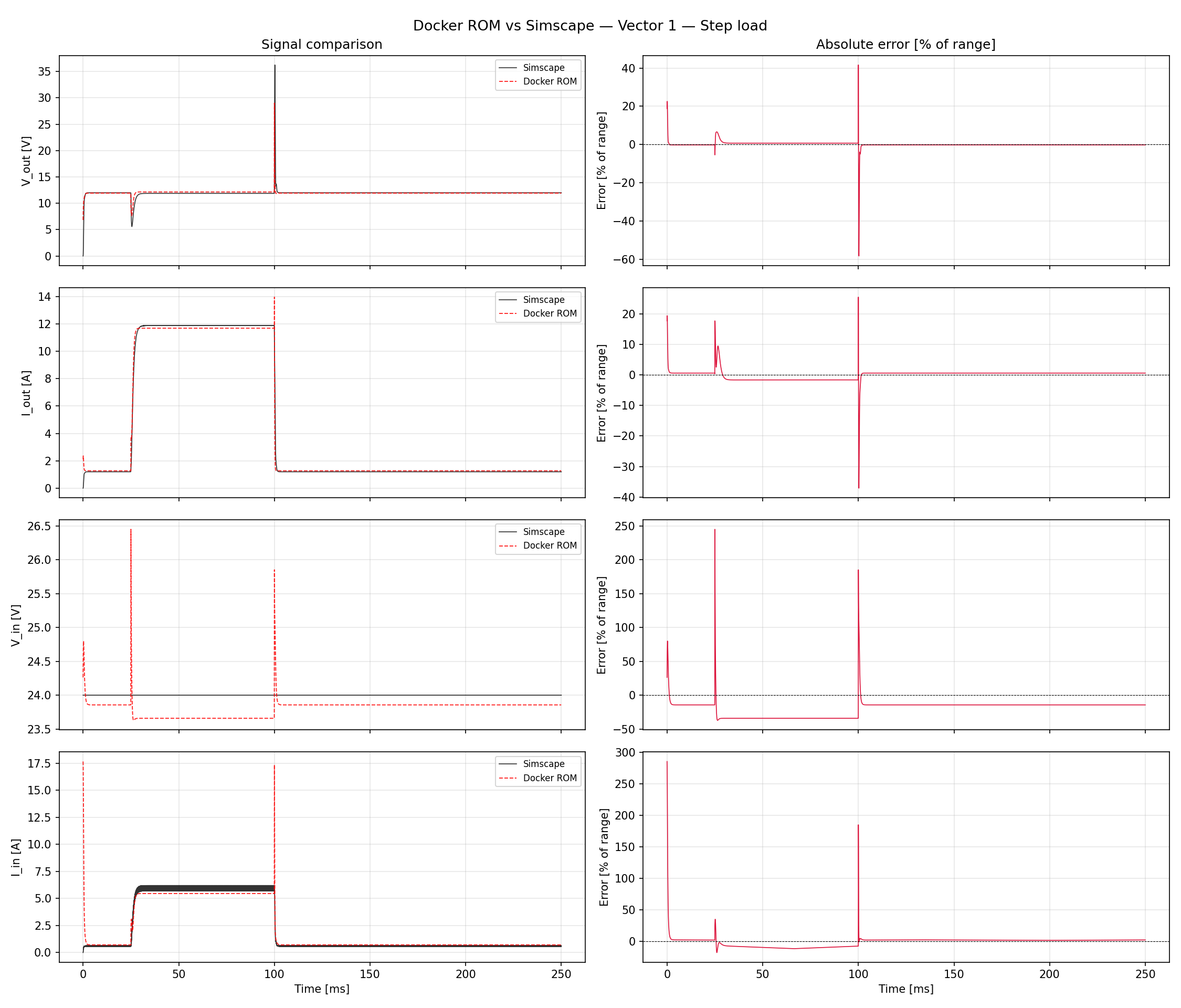
- $V_{out}$ dynamics: the ROM captures the inductive voltage dip and recovery during the $10\,\Omega \rightarrow 1\,\Omega$ load step.
- $I_{out}$ step: the current profile matches the reference with $1.07\%$ MAE.
Vector 2 - Ramp $V_{in}$ + Sinusoidal Duty Cycle
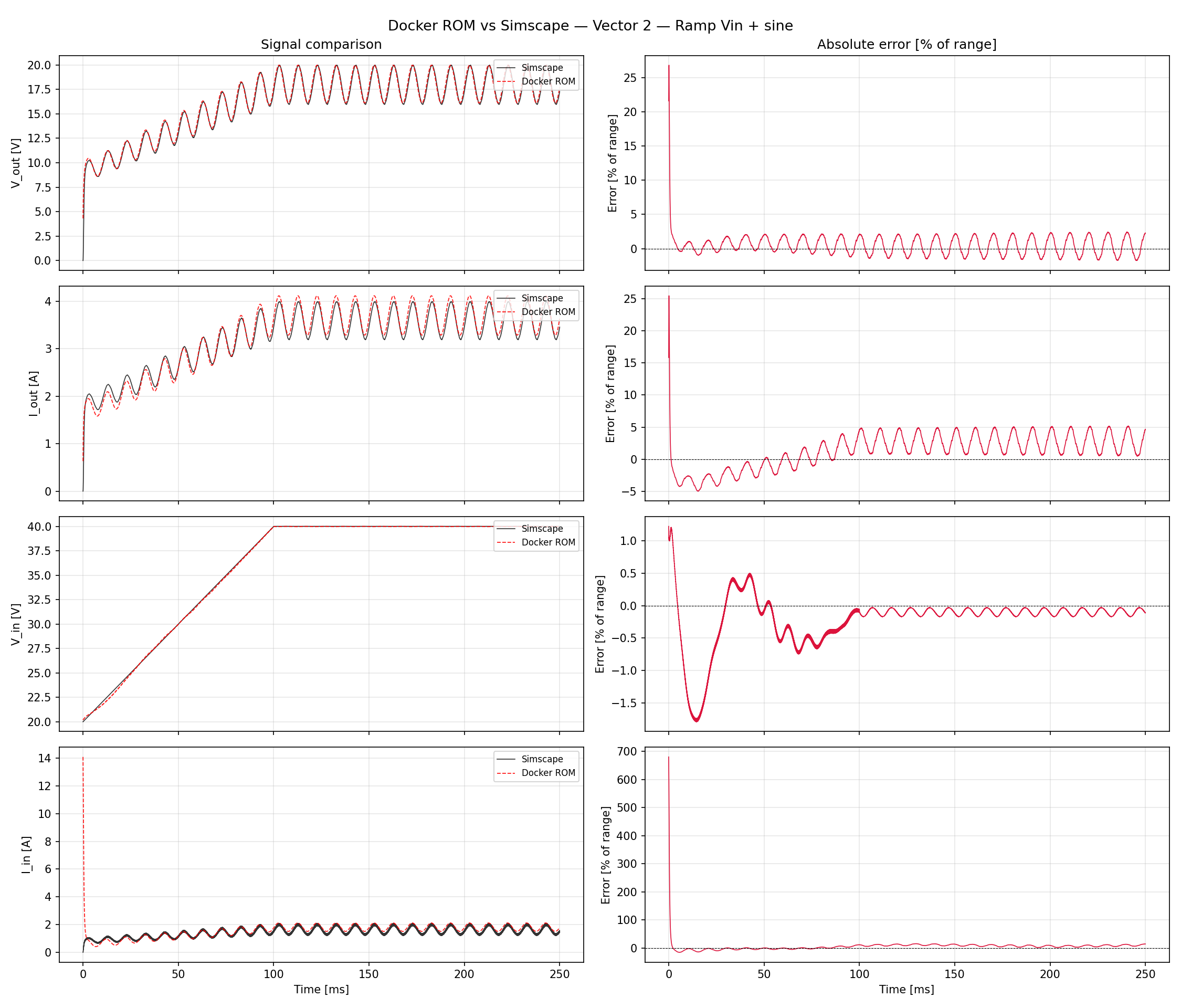
- Under simultaneous line voltage ramping ($20\,\text{V} \rightarrow 40\,\text{V}$) and $100\,\text{Hz}$ duty cycle perturbation, the ROM tracks both envelope and phase of $V_{out}$ and $I_{out}$.
6. Computational Efficiency
| Scenario | Physical Duration | Simscape Wall-clock | Simthetic ROM | Speedup |
|---|---|---|---|---|
| Vector 1 | $250\,\text{ms}$ | $23.38\,\text{s}$ | $765.4\,\text{ms}$ | 30.6× |
| Vector 2 | $250\,\text{ms}$ | $22.61\,\text{s}$ | $818.7\,\text{ms}$ | 27.6× |
Notes
- ROM time is the internal model execution time reported by the container; it does not include container startup (~1 s, one-time cost amortised across many runs) or HTTP overhead.
- Simscape was run on the same host under the solver settings in §2.
- The native C-library underlying the ROM can be linked directly into a host application (FFI, FMU, or embedded target) to remove the Docker/HTTP layer entirely.
7. Deployment Options
Docker REST API
Current benchmark setup: zero-install on Linux/Windows/macOS, language-agnostic via HTTP, no MATLAB or PyTorch licences required.
Embedded C Library
The ROM core compiles to a self-contained .dll / .so suitable for direct linkage in C/C++ host code or HIL platforms.
FMU Export
FMI-compliant package for integration with Simulink, Dymola, OpenModelica and similar tools.
8. Known Limitations
- Operating envelope: accuracy outside the ranges in §3 is not validated. The current ROM was not trained on transients that take any input variable across the boundary mid-simulation.
- $I_{in}$ transient accuracy: as detailed in §4 note ², the input-current trace shows larger relative deviation than the output-side signals, particularly at switching instants. Applications that close a control loop on $I_{in}$ should review the absolute error magnitudes for fit.
- Single-phase topology only: this ROM does not model multi-phase or interleaved Buck variants.