Headline numbers
| Quantity | Value |
|---|---|
| ROM time step | 50 µs |
| Inputs / outputs | 3 / 5 |
| ROM architecture | LSTM, 50-sample window, ~6k parameters |
| Accuracy (12 unseen trajectories) | 1.73 % of full scale (mean NRMSE) |
| Simscape reference | 517 µs per step at a 0.5 µs step (≈ 0.001× real-time) |
| ROM speed-up, desktop x86 | ~95,000× (92× real-time, standalone compiled C code) |
| ROM speed-up, MCU (Arm Cortex-M7) | ~4,000× (3.9× real-time) |
| x86 execution (float32) | 543 ns per step = 10.8 ns per simulated µs |
| MCU execution (int16) | 12.9 µs per 50 µs step |
| MCU worst-case execution time | 17,465 cycles = 43.7 µs |
Executive summary
In this paper, we model a 100 kHz LLC DC-DC converter in Simscape, which runs at about 0.001× real-time, and generate its reduced order model (ROM). The ROM runs about 4× faster than real time on a microcontroller, with a mean error of about 1.7 % of full scale.
The system and the reference model
An LLC DC-DC converter is a power electronics converter with a complex, nonlinear relationship between its inputs and outputs. Commonly used in computer power supplies, electric vehicle chargers and many other applications, it is a fundamental component of our everyday lives.
These converters operate at very high frequencies, which makes circuit simulation computationally heavy and slow, and limits how much design-space exploration engineers can afford.
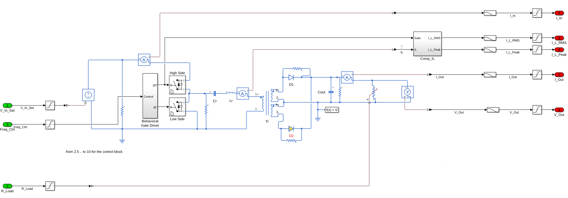
To model a generic LLC converter, we used a publicly available demo: the MathWorks DC-DC LLC Converter Simscape model.
We made some modifications on top of the original model:
- generated RMS and peak values of the resonant inductor current, rather than using its raw waveform;
- removed the PI controller;
- added resistors to help the solver;
- added a variable resistor as the load;
- bounded the inputs and outputs;
- low-pass filtered the outputs, with time constant \(T = 300\,\mu\mathrm{s}\).
| Parameter | Description | Value |
|---|---|---|
| \(T_s\) | Simulation sample time | 0.5 µs |
| \(f_r\) | Resonant frequency | 113.64 kHz |
| \(L_r\) | Resonant inductance | 162.26 µH |
| \(C_r\) | Resonant capacitance | 12.089 nF |
| \(V_{\mathrm{In,nom}}\) | Nominal input voltage | 450 V |
| \(V_{\mathrm{Out,nom}}\) | Nominal output voltage | 54 V |
Running this model in Simulink's Normal mode takes on average 517 µs of wall-clock time per step. That is about 1,030 seconds (17 minutes) of compute per simulated second on an Intel Core i5-8400 with 16 GB of RAM.
Why LLC resists naive surrogate modelling
The relationship between \(V_{\mathrm{Out}}\) and \(V_{\mathrm{In}}\) in an LLC converter is nonlinear: the voltage gain \(M\) is a nonlinear function of the switching frequency \(f_{\mathrm{sw}}\),
and, as the figure below shows, the shape of \(M\) itself changes with the load. The output current, in turn, is to a good approximation the output voltage divided by the load:
For a fixed load this is linear, but across an operating envelope spanning 10.9 to 100 Ω it is not, and no model that is affine in its inputs can represent it.
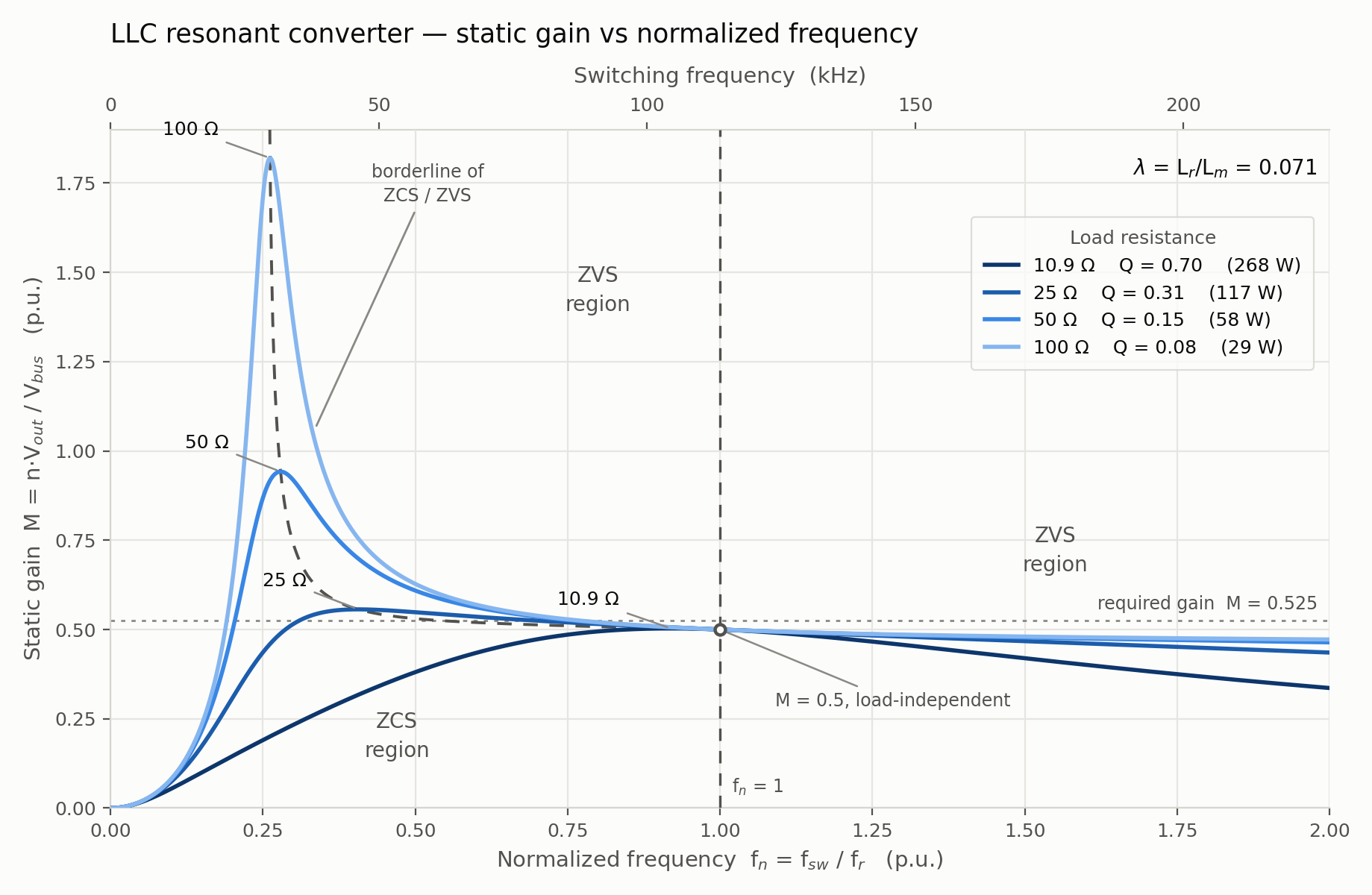
A simple model therefore cannot represent these relationships.
The switching frequency, around 100 kHz, is also extremely high: even though the envelopes of \(V_{\mathrm{Out}}\) and \(I_{\mathrm{Out}}\) are essentially DC, the underlying phenomena play out at the sub-microsecond level.
ROM architecture
The ROM has the following interfaces:
| Direction | Signal | Symbol | Description / range |
|---|---|---|---|
| Inputs | Freq_Ctrl | \(f\) | Switching frequency, \([0.59,\ 0.81]\,f_r\) (≈ 67–92 kHz) |
| V_In_Set | \(V_{\mathrm{In}}\) | Input voltage, \([250,\ 550]\) V | |
| R_Load | \(R_{\mathrm{Load}}\) | Load resistance, \([10.9,\ 100]\) Ω | |
| Outputs | I_In | \(I_{\mathrm{In}}\) | Input current (A) |
| I_L_Peak | \(I_{L,\mathrm{Peak}}\) | Resonant inductor peak current (A) | |
| I_L_RMS | \(I_{L,\mathrm{RMS}}\) | Resonant inductor RMS current (A) | |
| I_Out | \(I_{\mathrm{Out}}\) | Output current (A) | |
| V_Out | \(V_{\mathrm{Out}}\) | Output voltage (V) |
The ROM is composed of a few layers, including an LSTM with a 50-sample window, for a total of around 6,000 parameters.
Feature augmentation
The three physical inputs alone are not enough to describe their relationship with the outputs accurately, so feature augmentation is necessary. We artificially create new “inputs” that are functions of the existing physical inputs, giving the model more candidate relationships with the outputs.
These augmented features are detected automatically from a set of predefined functions and tested with a statistical screening. In short, if an augmented feature appears to add information that helps us model the outputs, we add it to the ROM.
The selected features are computed internally and are invisible to the user (\(f\) denotes Freq_Ctrl):
On their own, these 7 augmented features reduce the steady-state RMSE, compared with a non-augmented baseline, by 25.6 % (\(I_{\mathrm{Out}}\)), ~39 % (\(I_{L,\mathrm{Peak}}\) and \(I_{L,\mathrm{RMS}}\)), 52.8 % (\(I_{\mathrm{In}}\)) and 61.5 % (\(V_{\mathrm{Out}}\)).
Results
Errors are reported as NRMSE, the RMSE normalised by the output's full scale (its rated range):
The accuracy metrics at the 50 µs ROM update rate are:
| Metric | \(I_{\mathrm{In}}\) | \(I_{L,\mathrm{Peak}}\) | \(I_{L,\mathrm{RMS}}\) | \(I_{\mathrm{Out}}\) | \(V_{\mathrm{Out}}\) |
|---|---|---|---|---|---|
| NRMSE (% of full scale) | 0.62 | 1.88 | 1.87 | 1.30 | 2.98 |
| RMSE | 0.070 A | 0.067 A | 0.044 A | 0.078 A | 2.39 V |
| 95th-percentile abs. error | 0.082 A | 0.140 A | 0.087 A | 0.135 A | 5.34 V |
| Bias | +0.008 A | −0.004 A | +0.004 A | +0.014 A | +0.42 V |
| \(R^2\) | 0.63 | 0.960 | 0.961 | 0.989 | 0.974 |
| Split | Runs | Mean NRMSE (% of full scale) |
|---|---|---|
| Training | 32 | 1.78 |
| Validation | 8 | 2.42 |
| Test (unseen data) | 12 | 1.73 |
The figures below compare the ROM with the Simscape model on one of the unseen test runs, for each of the five outputs.
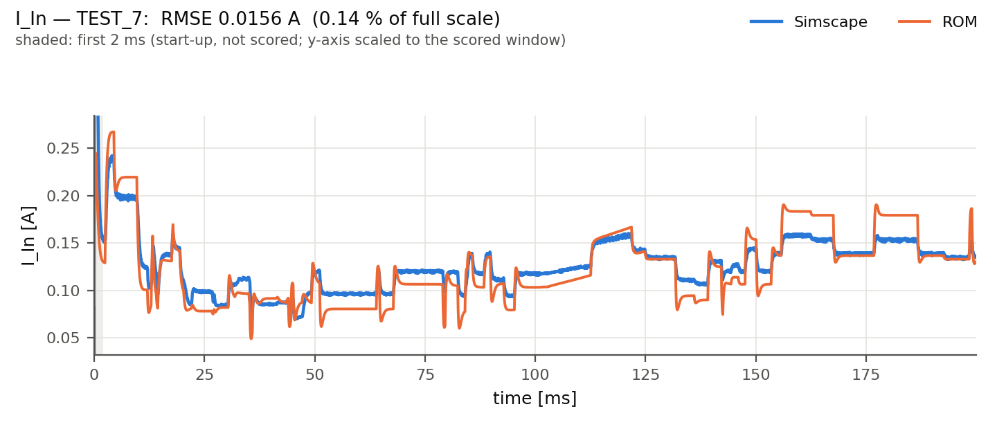
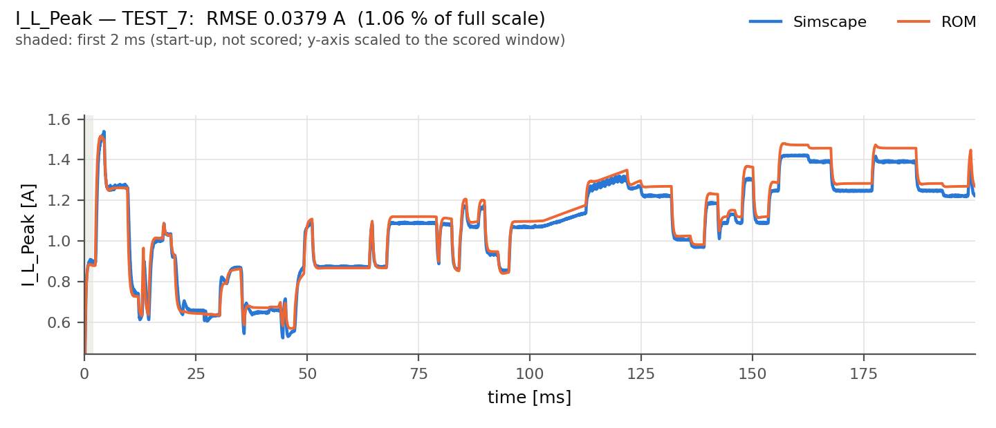
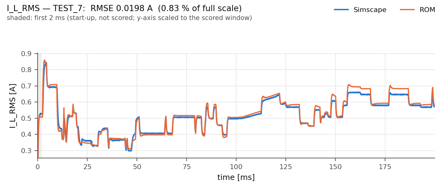
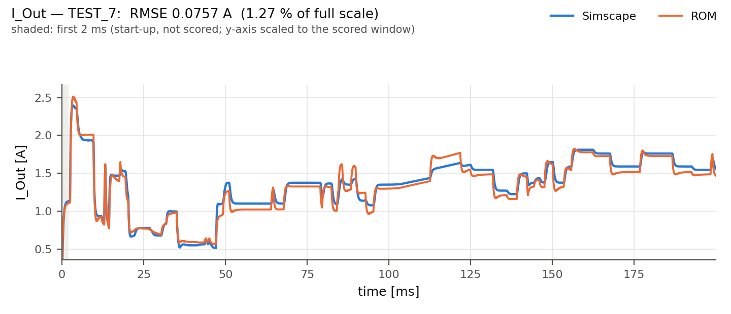
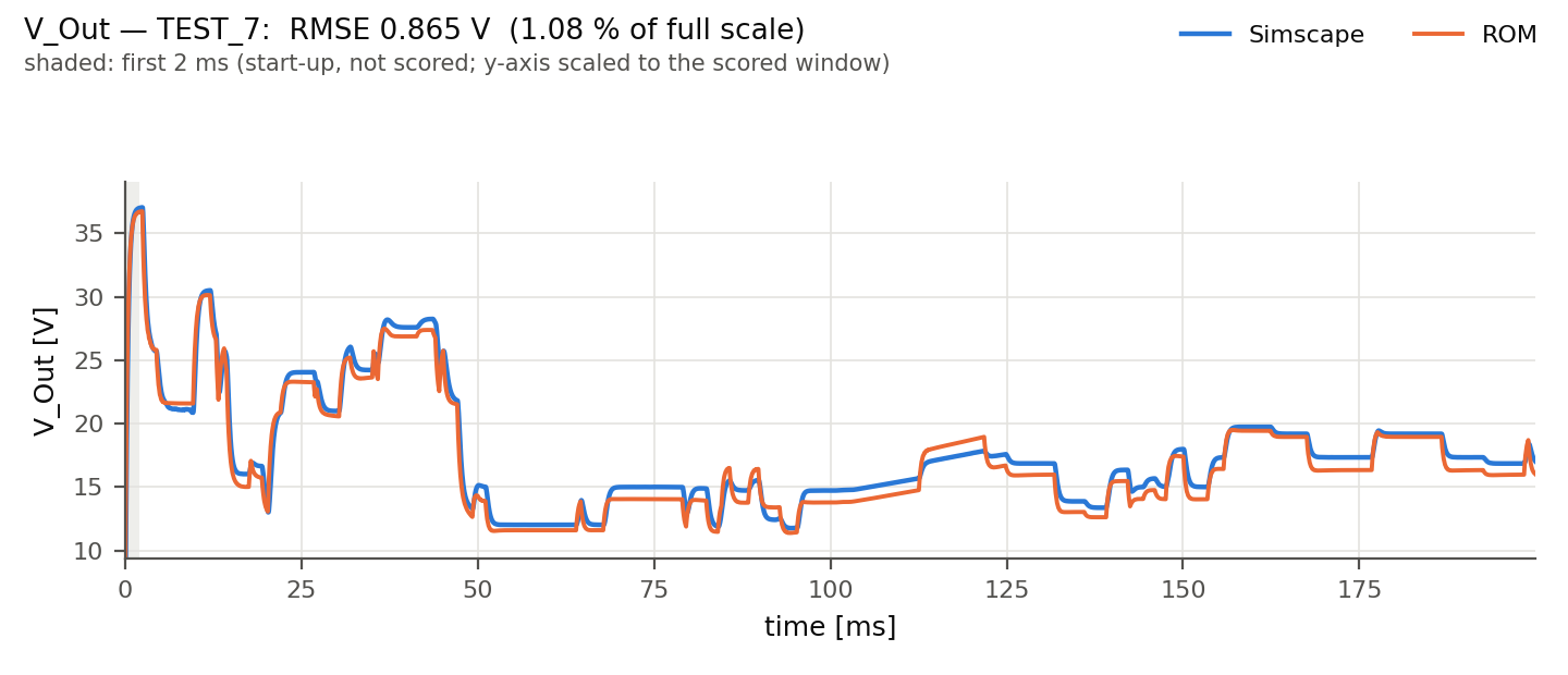
The low \(R^2\) for \(I_{\mathrm{In}}\) reflects the input capacitor's inrush current, which the ROM does not model. These are large-amplitude but short-lived events (several amps lasting a few milliseconds), and \(R^2\) penalises them heavily because it measures explained variance. The error distribution shows the same thing: 95 % of \(I_{\mathrm{In}}\) errors stay below 0.082 A, but the worst reaches 3.98 A, a factor of 48 higher. Away from input steps, \(I_{\mathrm{In}}\) is the most accurate output in the set, with the best NRMSE of all five at 0.62 % of full scale.
Choosing the ROM's time step
The reference Simscape model runs at a 0.5 µs step because it must resolve individual switching transitions. The ROM does not model switching; it models the envelope those transitions produce. Its own dynamics are therefore far slower: the identified model has characteristic time constants ranging from \(\tau_{\min} = 492\,\mu\mathrm{s}\) to roughly 3 ms.
This matters because our first ROM ran at a 1 µs step, inherited from the reference model's sample rate. That step oversampled the ROM's own fastest dynamics by roughly 500×. The ROM had inherited a constraint from physics it had deliberately discarded, and was paying for resolution it could not use.
We coarsened the step in two stages:
- 1 µs → 25 µs: faster and more accurate. The speed gain was expected; the accuracy gain was not. The model carries a 50-sample memory window, and at a 1 µs step that window spans only 50 µs, a tenth of the fastest time constant in the system, leaving it effectively blind to the dynamics it needs to capture. At 25 µs the same 50 samples span 1.25 ms and cover the dominant modes.
- 25 µs → 50 µs: a deliberate trade. 3.7× less compute per simulated second for roughly 14 % higher relative error. For a model intended to run alongside control software on an embedded target this was the right trade, and it is what brought the ROM inside the core-load budget described in Embedded deployment.
The ROM's internal update interval \(T\) cannot be stretched indefinitely. A value refreshed every \(T\) is frozen for \(T\) while the system it describes keeps evolving, so the update rate imposes an error floor that no model, however accurate, can go below:
| Internal update interval \(T\) | \(T/\tau_{\min}\) | Error floor (% of full scale) |
|---|---|---|
| 100 µs | 0.2 | 0.18 |
| 200 µs | 0.4 | 0.40 |
| 400 µs | 0.8 | 0.68 |
Error floor: the error an ideal model (exact at every update instant) still incurs purely from holding values constant between updates (zero-order hold).
The limit follows from the model's own time constants. Against the fastest time constant of 492 µs, a 200 µs interval gives \(T/\tau_{\min} \approx 0.4\), and the held value still tracks the mode. At 400 µs the ratio is 0.8, so the value stays frozen for nearly the entire lifetime of the mode it represents, and the floor alone would consume about a third of the model's total error budget. 200 µs is therefore the practical ceiling.
A useful property of this floor is that it predicts reality: halving the internal update rate raised the floor by 0.22 points and the measured end-to-end error by 0.24 points. The table can therefore be used to price a rate change before committing to a retrain.
Numerical precision
By default, the ROM is evaluated in float32: weights and internal states alike. This is fine on a desktop CPU, but on an MCU a fixed-point implementation can be faster, depending on the target's FPU.
So the question is: can we move to fixed point, keeping the accuracy while increasing the speed on the target MCU? The answer is yes.
On x86, moving to int16 actually made the ROM about 2× slower than the float32 version, which is explained by the sophisticated FPUs of modern desktop CPUs. On the Cortex-M7 (STM32), int16 made the ROM about 2× faster.
Putting all three sources of error on the same scale:
| Error source | Desktop build (float32) | MCU build (int16) |
|---|---|---|
| How far the ROM is from the Simscape model (NRMSE) | 1.73 | 1.73 |
| How much the number format changes the result | 0.00007 | 0.012 |
| How far the generated C is from the reference model | 0.001 | 0 (bit-identical) |
All figures in % of full scale. Rows 2 and 3 are worst-case over the validation set and a 120-second stress run.
The first row is the only one that matters. Everything the ROM loses by using smaller numbers, or by being translated into C, is at least 144× smaller than its disagreement with the Simscape model, and on the desktop build about 25,000× smaller. Neither is visible in the result.
One small caveat: the LSTM's cell state must remain int32, as internal testing showed that int16 saturates and produces errors of 0.28 % of full scale.
C-code generation
The C code is generated automatically from the model, and every build is verified against the reference implementation before release. The tolerance check is part of the generation pipeline, not a manual review step. For the MCU build this check is exact: because integer arithmetic is fully reproducible, the board and the desktop library produce bit-identical outputs, so the deployed code is not merely close to the validated model but numerically the same.
Embedded deployment
The target is a NUCLEO-H753ZI development board, with an Arm Cortex-M7 running at 400 MHz.
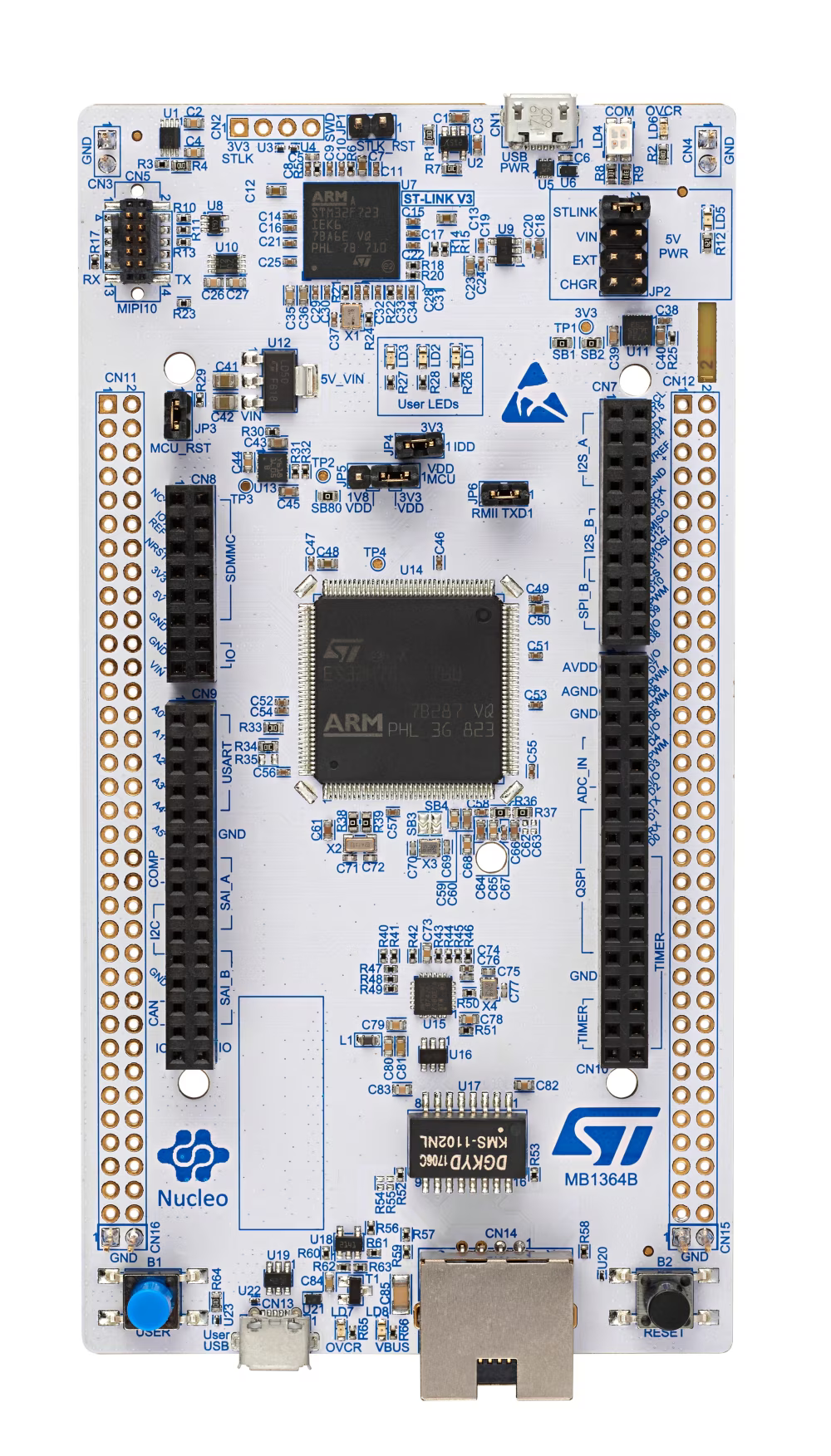
We tested the deployment with a webserver application running on a PC, which continuously sets the MCU's inputs and queries it for its status and outputs.
Internally, we set a target of 30 % core load, because the ROM is meant to run on the target alongside other software components, for example the actual control loop of the LLC converter. The timing results were:

Our C-code generation and embedded deployment guarantee deterministic timing, fixed loop bounds and no dynamic memory allocation, in line with what real-time systems expect.
Limitations and scope
- Outputs are invalid for roughly the first 500 µs from rest, as soft-start is not modelled.
- Simscape performance was only measured in Normal mode.
- The MCU build was tested with int16 weights, while the desktop build was tested with float32.
- The ROM is only valid within its training envelope; accuracy may degrade quickly outside that range.
What it enables
The ROM is not simply a faster version of the Simscape model. It is a different kind of artifact, and its applications follow from three properties the original does not have:
- it runs on a microcontroller;
- it runs faster than the converter itself (above real time);
- the code on the target is numerically identical to the code validated on a desktop.
On the target, alongside the control loop
At 26 % of one core, the ROM leaves room for the converter's actual control software on the same device. This enables:
- Virtual sensing. The ROM estimates \(I_{L,\mathrm{Peak}}\), \(I_{L,\mathrm{RMS}}\) and \(I_{\mathrm{In}}\) from \(f\), \(V_{\mathrm{In}}\) and \(R_{\mathrm{Load}}\) alone. The resonant inductor current is awkward and expensive to measure directly, yet its peak and RMS values are what drive magnetic and switch thermal stress. The ROM supplies both continuously, from signals the controller already has.
- Plausibility checking and fault detection. Running the ROM in parallel with the physical converter gives a continuously updated expectation for every output. A persistent divergence between measurement and prediction is itself a signal: component drift, a degraded capacitor or a failing sensor. This is the practical form of an edge digital twin, a reference the controller can compare itself against in real time.
- Lookahead. At 3.9× real-time the ROM simulates forward faster than the converter operates, so a controller can evaluate a commanded change before committing to it: for instance, whether a frequency transition would push the peak inductor current past its limit.
On the bench
On a desktop, the ROM covers one second of converter behaviour in 11 ms, against 17 minutes for the switching model. Studies that were previously uneconomic become routine: full-envelope sweeps across frequency, load and input voltage; Monte Carlo analysis over component tolerances; controller tuning against a plant that responds while you wait rather than overnight. The same model also runs in a hardware-in-the-loop (HIL) rig, something a switching Simscape model cannot do at any step size.
Across the workflow
Because the generated C is bit-identical between desktop and target, the model used for early design exploration, the one in the HIL rig and the one deployed on the ECU are the same model, not three approximations of one another. A result validated once stays valid along the whole chain, which removes a class of integration surprises that normally surface late.